CS 6.006 笔记

发表于 2024/02/25 更新于 2024/02/26

作者 cfbreathing 19 分钟 阅读

Lecture 01:Introduction

Problem

Binary relation from problem inputs to correct outputs
Usually don’t specify every correct output for all inputs (too many!)
Provide a verifiable predicate (a property) that correct outputs must satisfy
6.006 studies problems on large general input spaces
Not general: small input instance - Example: In this room, is there a pair of students with same birthday?
General: arbitrarily large inputs - Example: Given any set of n students, is there a pair of students with same birthday? - If birthday is just one of 365, for n > 365, answer always true by pigeon-hole - Assume resolution of possible birthdays exceeds n (include year, time, etc.)

Algorithm

Procedure mapping each input to a single output (deterministic)
Algorithm solves a problem if it returns a correct output for every problem input - Example: An algorithm to solve birthday matching
Maintain a record of names and birthdays (initially empty)
Interview each student in some order - If birthday exists in record, return found pair! - Else add name and birthday to record - Return None if last student interviewed without success

Correctness

Programs/algorithms have fixed size, so how to prove correct?
For small inputs, can use case analysis
For arbitrarily large inputs, algorithm must be recursive or loop in some way
Must use induction (why recursion is such a key concept in computer science)
Example: Proof of correctness of birthday matching algorithm - Induct on $k$: the number of students in record - Hypothesis: if first $k$ contain match, returns match before interviewing student $k + 1$ - Base case: $k = 0$, first $k$ contains no match - Assume for induction hypothesis holds for $k = k_0$ , and consider $k = k_0 + 1$ - If first $k_0$ contains a match, already returned a match by induction - Else first $k_0$ do not have match, so if first $k_0 + 1$ has match, match contains $k_0 + 1$ - Then algorithm checks directly whether birthday of student $k_0 + 1$ exists in first $k_0$

Efficiency

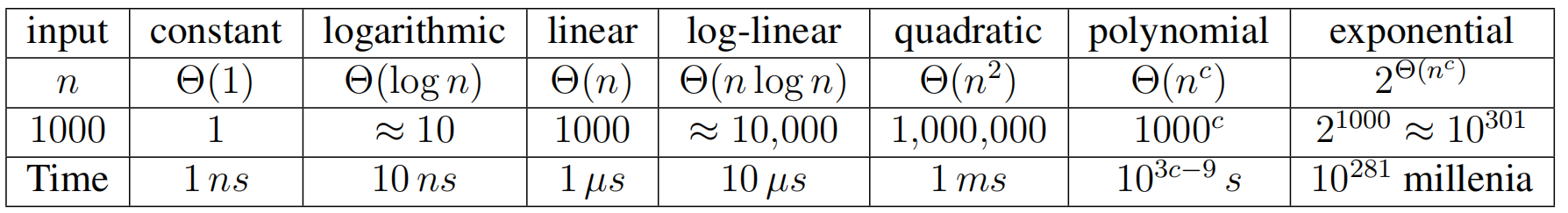
How fast does an algorithm produce a correct output? - Could measure time, but want performance to be machine independent - Idea! Count number of fixed-time operations algorithm takes to return - Expect to depend on size of input: larger input suggests longer time - Size of input is often called ‘n’, but not always! - Efficient if returns in polynomial time with respect to input - Sometimes no efficient algorithm exists for a problem! (See L20)
Asymptotic Notation: ignore constant factors and low order terms - Upper bounds (O), lower bounds (Ω), tight bounds (Θ) - Time estimate below based on one operation per cycle on a 1 GHz single-core machine - Particles in universe estimated < $10^{100}$

1 def birthday_match(students):
2 ’’’
3 Find a pair of students with the same birthday
4 Input: tuple of student (name, bday) tuples
5 Output: tuple of student names or None
6 ’’’
7 n = len(students) # O(1)
8 record = StaticArray(n) # O(n)
9 for k in range(n): # n
10 (name1, bday1) = students[k] # O(1)
11 # Return pair if bday1 in record
12 for i in range(k): # k
13 (name2, bday2) = record.get_at(i) # O(1)
14 if bday1 == bday2: # O(1)
15 return (name1, name2) # O(1)
16 record.set_at(k, (name1, bday1)) # O(1)
17 return None # O(1)

Example: Running Time Analysis

Two loops: outer $k \in {0, . . . , n − 1}$, inner is $i \in{0, . . . , k}$Pn−1
Running time is $O(n) + \sum_{k=0}^{n-1}(O(1) + k \cdot O(1)) = O(n^2)$
Quadratic in n is polynomial. Efficient? Use different data structure for record!

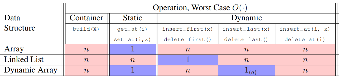
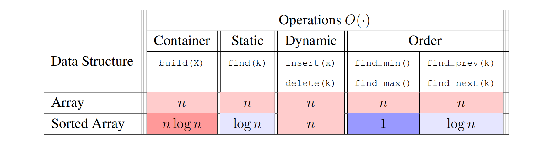
Lecture 2: Data Structures

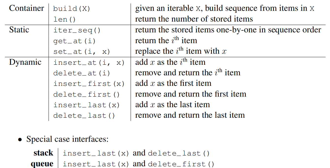
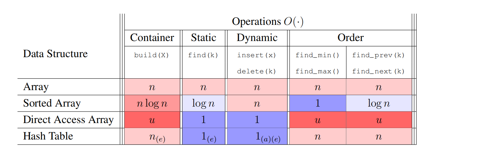
Data Structure Interfaces

A data structure is a way to store data, with algorithms that support operations on the data
Collection of supported operations is called an interface (also API or ADT)
Interface is a specification: what operations are supported (the problem!)
Data structure is a representation: how operations are supported (the solution!)
In this class, two main interfaces: Sequence and Set

Sequence Interface (L02, L07)

Maintain a sequence of items (order is extrinsic)
Ex: $(x_0, x_1, x_2, . . . , x_{n−1})$ (zero indexing)
(use $n$ to denote the number of items stored in the data structure)
Supports sequence operations:

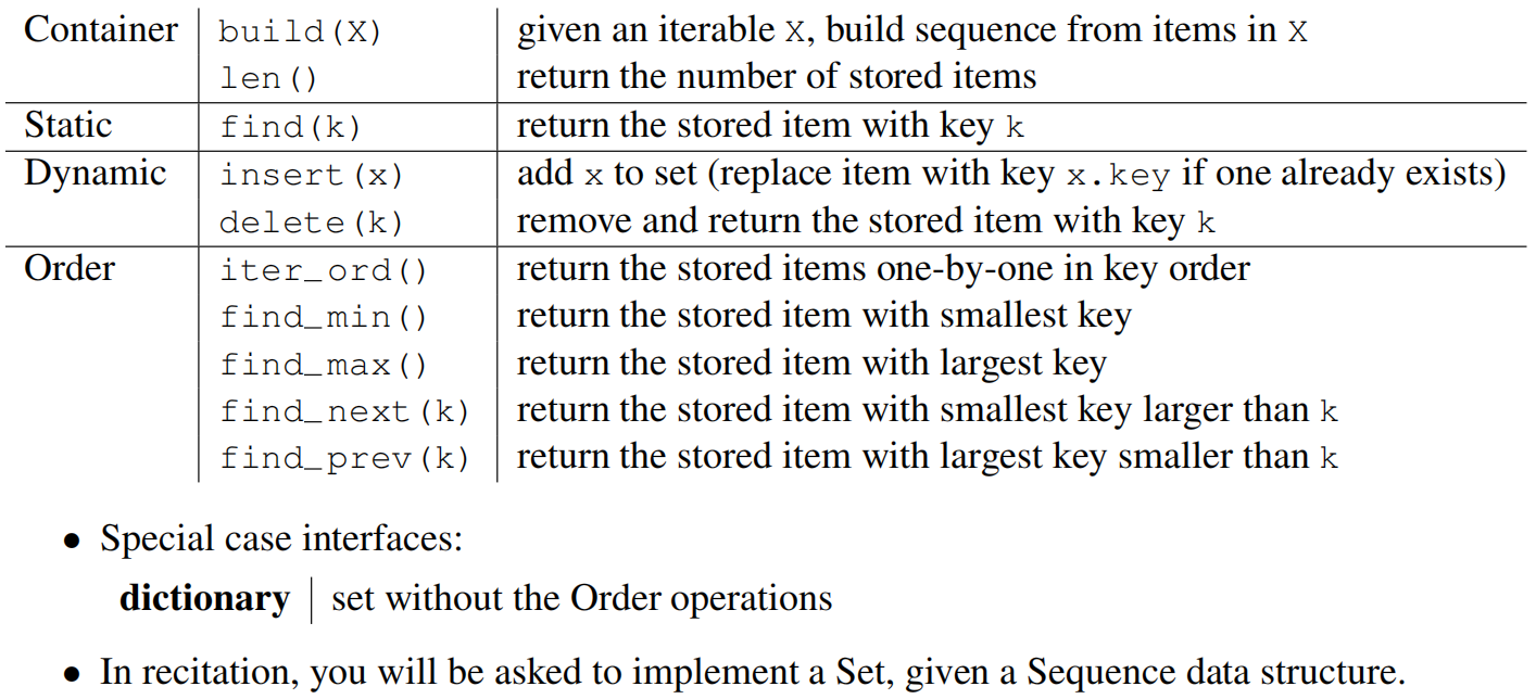
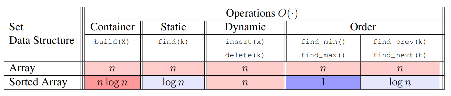
Set Interface (L03-L08)

Sequence about extrinsic order, set is about intrinsic order
Maintain a set of items having unique keys (e.g., item x has key x.key)
(Set or multi-set? We restrict to unique keys for now.)
Often we let key of an item be the item itself, but may want to store more info than just key
Supports set operations:

Dynamic Array Deletion

Delete from back? $\Theta(1)$ time without effort, yay!
However, can be very wasteful in space. Want size of data structure to stay $\Theta(n)$
Attempt: if very empty, resize to $r = 1$. Alternating insertion and deletion could be bad…
Idea! When $r < r_d$, resize array to ratio $r_i$ where $r_d < r_i$ (e.g., $r_d = 1/4$, $r_i = 1/2$)
Then $\Theta(n)$ cheap operations must be made before next expensive resize
Can limit extra space usage to $(1 + \varepsilon)n$ for any $\varepsilon > 0$ (set $r_d = \frac{1}{1+\varepsilon}$, $r_i = \frac{r_d+1}{2}$)
Dynamic arrays only support dynamic last operations in $\Theta(1)$ time
Python List append and pop are amortized $O(1)$ time, other operations can be $O(n)$!
(Inserting/deleting efficiently from front is also possible; you will do this in PS1)

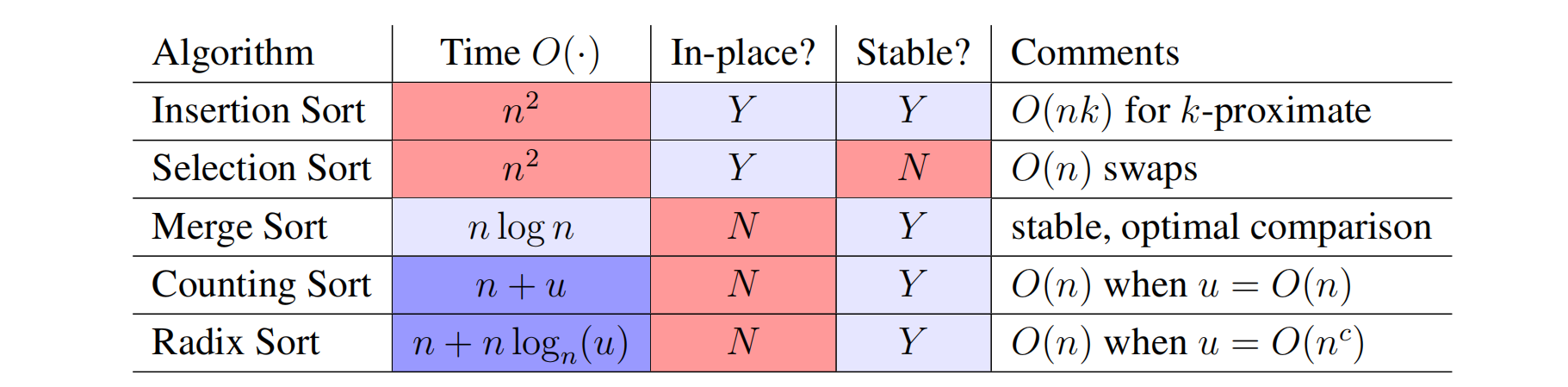
Lecture 3: Sorting

Sorting

Given a sorted array, we can leverage binary search to make an efficient set data structure.
Input: (static) array A of n numbers
Output: (static) array B which is a sorted permutation of A - Permutation: array with same elements in a different order - Sorted: B[i − 1] ≤ B[i] for all i ∈ {1, . . . , n}
Example: [8, 2, 4, 9, 3] → [2, 3, 4, 8, 9]
A sort is destructive if it overwrites A (instead of making a new array B that is a sorted version of A)
A sort is in place if it uses O(1) extra space (implies destructive: in place ⊆ destructive)

Permutation Sort

There are n! permutations of A, at least one of which is sorted
For each permutation, check whether sorted in $\Theta(n)$
Example: [2, 3, 1] → {[1, 2, 3], [1, 3, 2], [2, 1, 3], [2, 3, 1], [3, 1, 2], [3, 2, 1]}

1 def permutation_sort(A):
2 ’’’Sort A’’’
3 for B in permutations(A): # O(n!)
4 if is_sorted(B): # O(n)
5 return B # O(1)

permutation sort analysis: - Correct by case analysis: try all possibilities (Brute Force) - Running time: Ω(n! · n) which is exponential

Solving Recurrences

Substitution: Guess a solution, replace with representative function, recurrence holds true
Recurrence Tree: Draw a tree representing the recursive calls and sum computation at nodes
Master Theorem: A formula to solve many recurrences (R03)

Selection Sort

Find a largest number in prefix A[:i + 1] and swap it to A[i]
Recursively sort prefix A[:i]
Example: [8, 2, 4, 9, 3], [8, 2, 4, 3, 9], [3, 2, 4, 8, 9], [3, 2, 4, 8, 9], [2, 3, 4, 8, 9]

 def selection_sort(A, i = None): # T(i)
2 ’’’Sort A[:i + 1]’’’
3 if i is None: i = len(A) - 1 # O(1)
4 if i > 0: # O(1)
5 j = prefix_max(A, i) # S(i)
6 A[i], A[j] = A[j], A[i] # O(1)
7 selection_sort(A, i - 1) # T(i - 1)
8
9 def prefix_max(A, i): # S(i)
10 ’’’Return index of maximum in A[:i + 1]’’’
11 if i > 0: # O(1)
12 j = prefix_max(A, i - 1) # S(i - 1)
13 if A[i] < A[j]: # O(1)
14 return j # O(1)
15 return i # O(1)

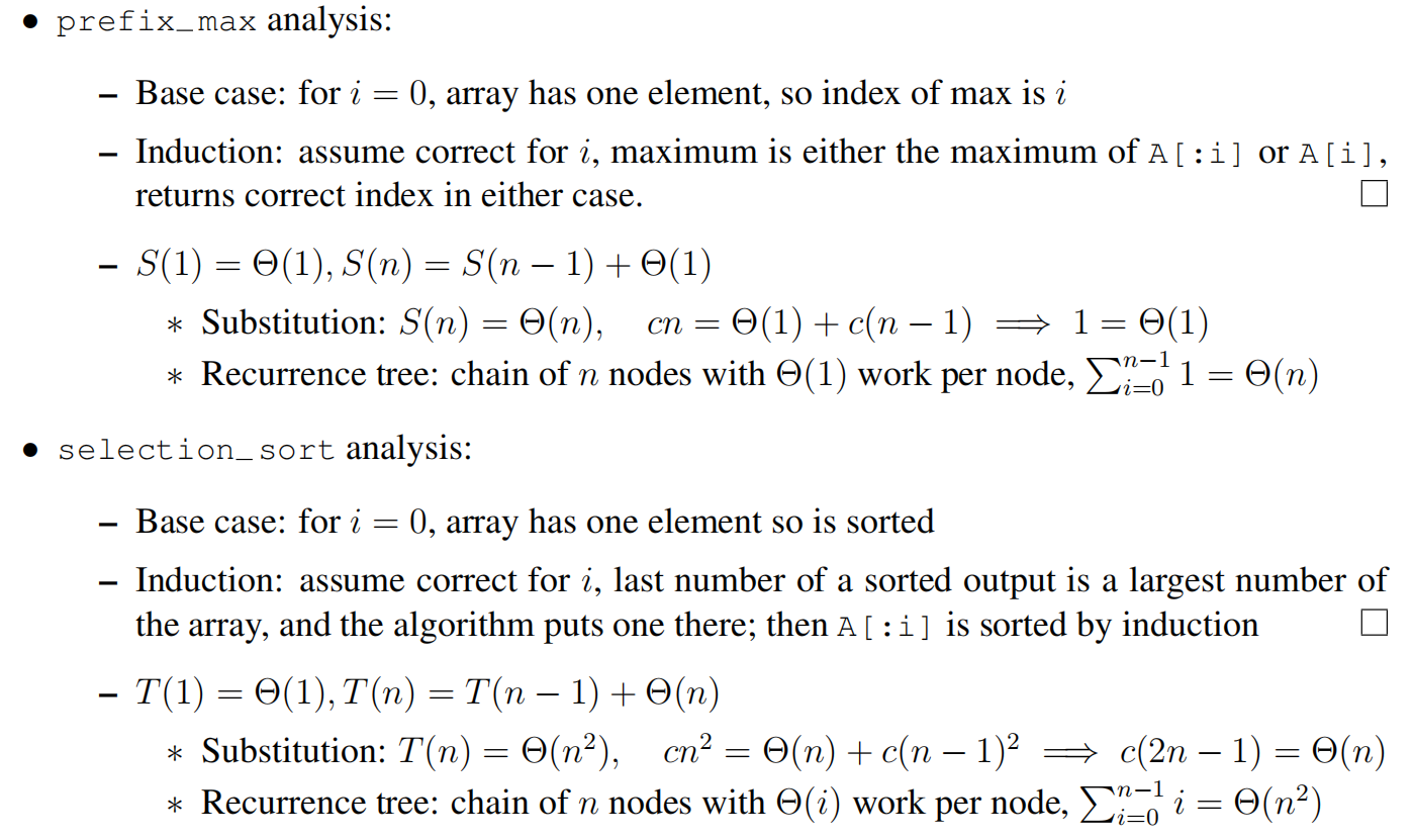
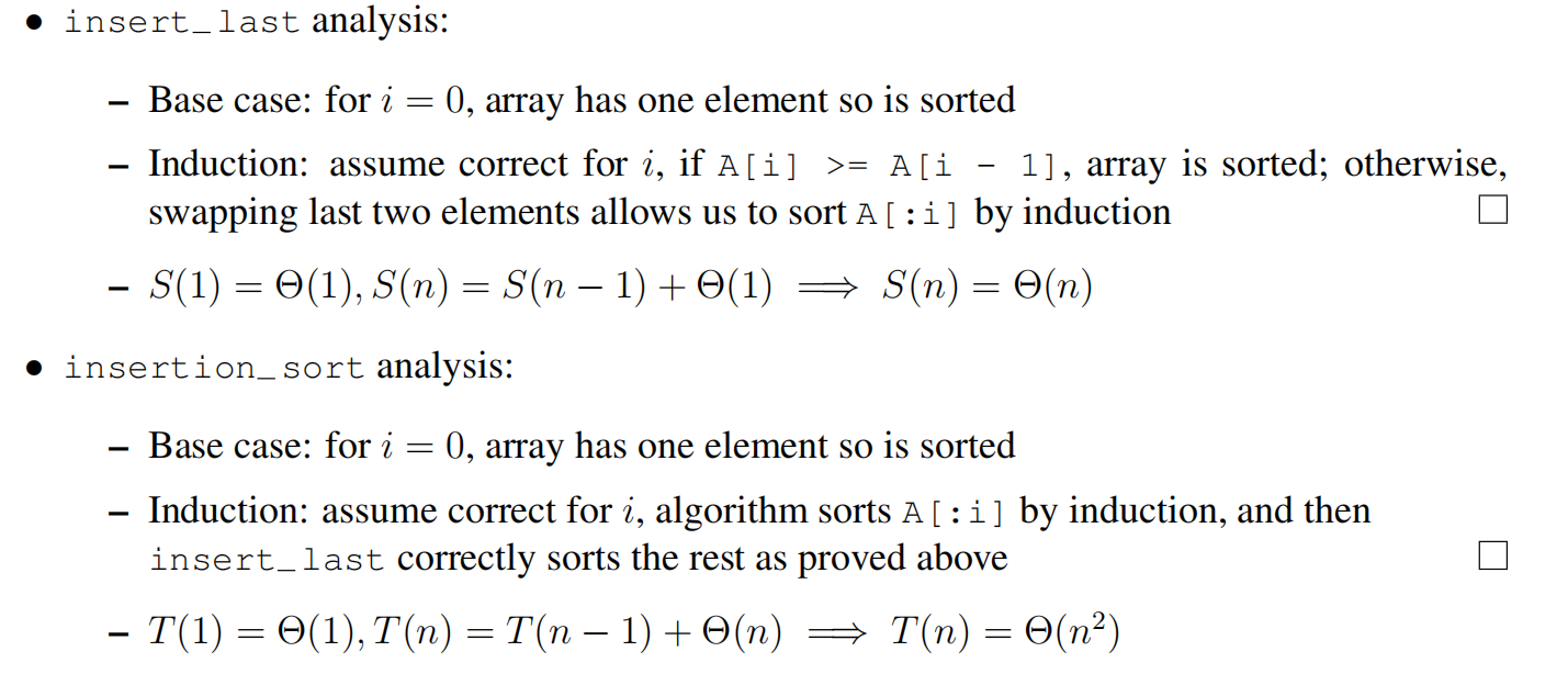
Insertion Sort

Recursively sort prefix A[:i]
Sort prefix A[:i + 1] assuming that prefix A[:i] is sorted by repeated swaps
Example: [8, 2, 4, 9, 3], [2, 8, 4, 9, 3], [2, 4, 8, 9, 3], [2, 4, 8, 9, 3], [2, 3, 4, 8, 9]

1 def insertion_sort(A, i = None): # T(i)
2 ’’’Sort A[:i + 1]’’’
3 if i is None: i = len(A) - 1 # O(1)
4 if i > 0: # O(1)
5 insertion_sort(A, i - 1) # T(i - 1)
6 insert_last(A, i) # S(i)
7
8 def insert_last(A, i): # S(i)
9 ’’’Sort A[:i + 1] assuming sorted A[:i]’’’
10 if i > 0 and A[i] < A[i - 1]: # O(1)
11 A[i], A[i - 1] = A[i - 1], A[i] # O(1)
12 insert_last(A, i - 1) # S(i - 1)

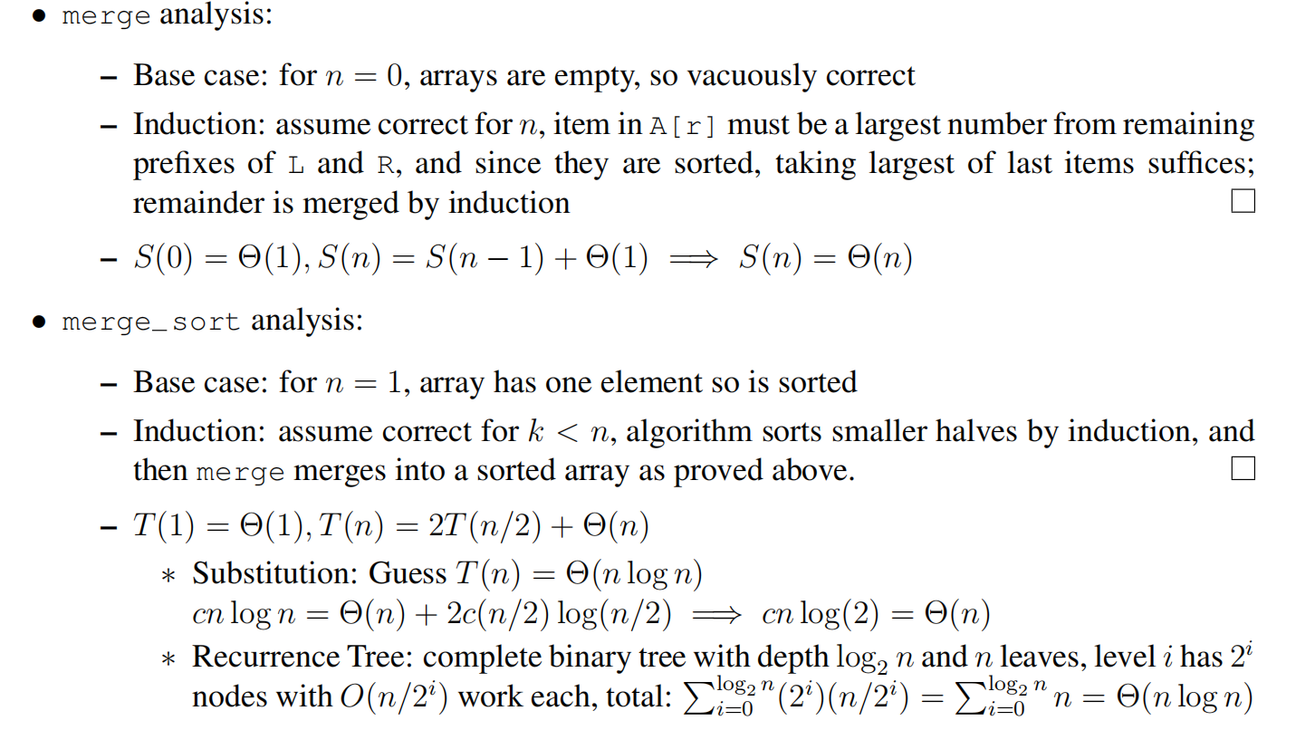
Merge Sort

Recursively sort first half and second half (may assume power of two)
Merge sorted halves into one sorted list (two finger algorithm)
Example: [7, 1, 5, 6, 2, 4, 9, 3], [1, 7, 5, 6, 2, 4, 3, 9], [1, 5, 6, 7, 2, 3, 4, 9], [1, 2, 3, 4, 5, 6, 7, 9]

1 def merge_sort(A, a = 0, b = None): # T(b - a = n)
2 ’’’Sort A[a:b]’’’
3 if b is None: b = len(A) # O(1)
4 if 1 < b - a: # O(1)
5 c = (a + b + 1) // 2 # O(1)
6 merge_sort(A, a, c) # T(n / 2)
7 merge_sort(A, c, b) # T(n / 2)
8 L, R = A[a:c], A[c:b] # O(n)
9 merge(L, R, A, len(L), len(R), a, b) # S(n)
10
11 def merge(L, R, A, i, j, a, b): # S(b - a = n)
12 ’’’Merge sorted L[:i] and R[:j] into A[a:b]’’’
13 if a < b: # O(1)
14 if (j <= 0) or (i > 0 and L[i - 1] > R[j - 1]): # O(1)
15 A[b - 1] = L[i - 1] # O(1)
16 i = i - 1 # O(1)
17 else: # O(1)
18 A[b - 1] = R[j - 1] # O(1)
19 j = j - 1 # O(1)
20 merge(L, R, A, i, j, a, b - 1) # S(n - 1)

Master Theorem

The Master Theorem provides a way to solve recurrence relations in which recursive calls decrease problem size by a constant factor. Given a recurrence relation of the form $T(n) = aT(n/b)+ f(n)$ and $T(1) = Θ(1)$, with branching factor $a ≥ 1$, problem size reduction factor $b > 1$, and asymptotically non-negative function $f(n)$, the Master Theorem gives the solution to the recurrence by comparing $f(n)$ to $a^{log_bn} = n^{log_b a}$, the number of leaves at the bottom of the recursion tree. When $f(n)$ grows asymptotically faster than $n^{log_b a}$, the work done at each level decreases geometrically so the work at the root dominates; alternatively, when $f(n)$ grows slower, the work done at each level increases geometrically and the work at the leaves dominates. When their growth rates are comparable, the work is evenly spread over the tree’s $O(log\;n)$ levels.

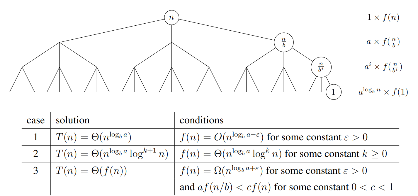
The Master Theorem takes on a simpler form when $f(n)$ is a polynomial, such that the recurrence has the from $T(n) = aT(n/b) + Θ(n^c)$ for some constant c ≥ 0.

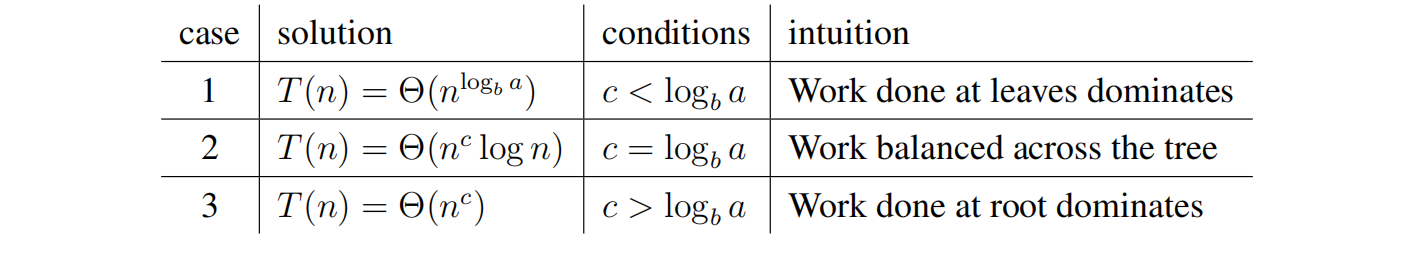
This special case is straight-forward to prove by substitution (this can be done in recitation). To apply the Master Theorem (or this simpler special case), you should state which case applies, and show that your recurrence relation satisfies all conditions required by the relevant case. There are even stronger (more general) formulas1 to solve recurrences, but we will not use them in this class.

Lecture 4: Hashing

Comparison Model

In this model, assume algorithm can only differentiate items via comparisons
Comparable items: black boxes only supporting comparisons between pairs
Comparisons are $<, ≤, >, ≥, \neq, =$, outputs are binary: True or False
Goal: Store a set of n comparable items, support find(k) operation
Running time is lower bounded by # comparisons performed, so count comparisons!

Decision Tree

Any algorithm can be viewed as a decision tree of operations performed
An internal node represents a binary comparison, branching either True or False
For a comparison algorithm, the decision tree is binary (draw example)
A leaf represents algorithm termination, resulting in an algorithm output
A root-to-leaf path represents an execution of the algorithm on some input
Need at least one leaf for each algorithm output, so search requires ≥ n + 1 leaves

Comparison Search Lower Bound

What is worst-case running time of a comparison search algorithm?
running time ≥ # comparisons ≥ max length of any root-to-leaf path ≥ height of tree
What is minimum height of any binary tree on ≥ n nodes?
Minimum height when binary tree is complete (all rows full except last)
Height $\geq\lceil lg(n + 1)\rceil − 1 = Ω(log\;n)$, so running time of any comparison sort is $Ω(log\;n)$
Sorted arrays achieve this bound! Yay!
More generally, height of tree with $Θ(n)$ leaves and max branching factor b is $Ω(log_b n)$
To get faster, need an operation that allows super-constant $ω(1)$ branching factor. How??

Direct Access Array

Exploit Word-RAM $O(1)$ time random access indexing! Linear branching factor!
Idea! Give item unique integer key $k$ in ${0, . . . , u − 1}$, store item in an array at index $k$
Associate a meaning with each index of array
If keys fit in a machine word, i.e. $u ≤ 2^w$, worst-case $O(1)$ find/dynamic operations! Yay!
Anything in computer memory is a binary integer, or use (static) 64-bit address in memory
But space $O(u)$, so really bad if $n \ll u$… :(
Example: if keys are ten-letter names, for one bit per name, requires $26^{10} ≈ 17.6 TB$ space
How can we use less space?

Hashing

Idea! If $n \ll u$, map keys to a smaller range $m = Θ(n)$ and use smaller direct access array
Hash function: $h(k) : {0, . . . , u - 1} → {0, . . . , m - 1}$ (also hash map)
Direct access array called hash table, h(k) called the hash of key k
If $m \ll u$, no hash function is injective by pigeonhole principle
Always exists keys a, b such that h(a) = h(b) → Collision! :(
Can’t store both items at same index, so where to store? Either: - store somewhere else in the array (open addressing) - complicated analysis, but common and practical - store in another data structure supporting dynamic set interface (chaining)

Chaining

Idea! Store collisions in another data structure (a chain)
If keys roughly evenly distributed over indices, chain size is $n/m = n/Ω(n) = O(1)$ - If chain has $O(1)$ size, all operations take $O(1)$ time! Yay!
If not, many items may map to same location, e.g. $h(k)$ = constant, chain size is $Θ(n)$ :(
Need good hash function! So what’s a good hash function?

Hash Functions

Division (bad): $h(k) = k\;mod\;m$

Heuristic, good when keys are uniformly distributed!
$m$ should avoid symmetries of the stored keys
Large primes far from powers of 2 and 10 can be reasonable
Python uses a version of this with some additional mixing
If $u \gg n$, every hash function will have some input set that will a create $O(n)$ size chain
Idea! Don’t use a fixed hash function! Choose one randomly (but carefully)!

Universal (good, theoretically): $h_{ab}(k) = (((ak + b)\;mod\;p)\;mod\;m)$

Hash Family $\mathcal{H}(p, m) = {h_{ab} a, b \in {0, . . . , p -1}\;and\;a \neq 0}$
Parameterized by a fixed prime $p > u$, with a and b chosen from range ${0, . . . , p - 1}$
$\mathcal{H}$ is a Universal family: $Pr_{h\in H} {h(k_i) = h(k_j)} \leq 1/m\;\;\;\;\forall k_i \neq k_j \in {0, … , u -1}$
Why is universality useful? Implies short chain lengths! (in expectation)
$X_{ij}$ indicator random variable over $h \in \mathcal{H}: X_{ij} = 1\;\;if\;h(k_i) = h(k_j ), X_{ij} = 0$ otherwise
Size of chain at index $h(k_i)$ is random variable $X_i = \sum_j X_{ij}$
Expected size of chain at index $h(k_i)$

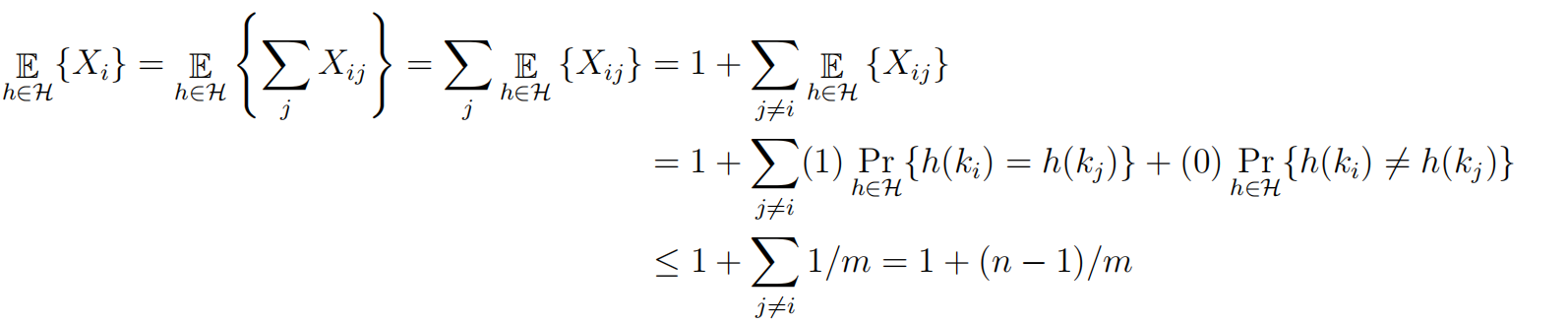
Since $m = \Omega(n)$, load factor $\alpha = n/m = O(1)$, so $O(1)$ in expectation!

Dynamic

If $n/m$ far from 1, rebuild with new randomly chosen hash function for new size m
Same analysis as dynamic arrays, cost can be amortized over many dynamic operations
So a hash table can implement dynamic set operations in expected amortized $O(1)$ time! :)

Lecture 5: Linear Sorting

Direct Access Array Sort

Example: [5, 2, 7, 0, 4]
Suppose all keys are unique non-negative integers in range {0, . . . , u − 1}, so n ≤ u
Insert each item into a direct access array with size u in $Θ(n)$
Return items in order they appear in direct access array in $Θ(u)$
Running time is $Θ(u)$, which is $Θ(n)$ if $u = Θ(n)$. Yay!

def direct_access_sort(A):
 u = 1 + max([x.key for x in A])
 D = [None] * u
 for x in A:
  D[x.key] = x
 i = 0
 for key in range(u):
  if D[key] is not None:
   A[i] = D[key]
   i += 1

What if keys are in larger range, like $u = Ω(n^2) < n^2$?
Idea! Represent each key $k$ by tuple $(a, b)$ where $k = an + b$ and $0 ≤ b < n$
Specifically $a = bk/nc < n$ and $b = (k mod n)$ (just a 2-digit base-n number!)
This is a built-in Python operation (a, b) = divmod(k, n)
Example: [17, 3, 24, 22, 12] ⇒ [(3,2), (0,3), (4,4), (4,2), (2,2)] ⇒ [32, 03, 44, 42, 22](n=5)
How can we sort tuples?

Tuple Sort

Item keys are tuples of equal length, i.e. item $x.key = (x.k1, x.k2, x.k2, . . .)$.
Want to sort on all entries lexicographically, so first key k1 is most significant
How to sort? Idea! Use other auxiliary sorting algorithms to separately sort each key
(Like sorting rows in a spreadsheet by multiple columns)
What order to sort them in? Least significant to most significant!
Exercise: [32, 03, 44, 42, 22] =⇒ [42, 22, 32, 03, 44] =⇒ [03, 22, 32, 42, 44](n=5)
Idea! Use tuple sort with auxiliary direct access array sort to sort tuples (a, b).
Problem! Many integers could have the same a or b value, even if input keys distinct
Need sort allowing repeated keys which preserves input order
Want sort to be stable: repeated keys appear in output in same order as input
Direct access array sort cannot even sort arrays having repeated keys!
Can we modify direct access array sort to admit multiple keys in a way that is stable?

Counting Sort

Instead of storing a single item at each array index, store a chain, just like hashing!
For stability, chain data structure should remember the order in which items were added
Use a sequence data structure which maintains insertion order
To insert item x, insert last to end of the chain at index x.key
Then to sort, read through all chains in sequence order, returning items one by one

  
def counting_sort(A):
 u = 1 + max([x.key for x in A])
 D = [[] for i in range(u)]
 for x in A:
  D[x.key].append(x)
 i = 0
 for chain in D:
  for x in chain:
   A[i] = x
   i += 1

There’s another implementation of counting sort which just keeps track of how many of each key map to each index, and then moves each item only once, rather the implementation above which moves each item into a chain and then back into place. The implementation below computes the final index location of each item via cumulative sums.

def conuting_sort(A):
 u = 1 + max([x.key for x in A])
 D = [0] * u
 for x in A:
  D[x.key] += 1
 for k in range(1, u):
  D[k] += D[k-1]
 for x in list(reversed(A)):
  A[D[x.key] - 1] = x
  D[x.key] -= 1

Radix Sort

Idea! If $u < n^2$, use tuple sort with auxiliary counting sort to sort tuples (a, b)
Sort least significant key b, then most significant key a
Stability ensures previous sorts stay sorted
Running time for this algorithm is $O(2n) = O(n)$. Yay!
If every key $< n^c$ for some positive $c = log_n(u)$, every key has at most c digits base n
A c-digit number can be written as a c-element tuple in O(c) time
We sort each of the c base-n digits in $O(n)$ time
So tuple sort with auxiliary counting sort runs in $O(cn)$ time in total
If c is constant, so each key is $≤ nc^$, this sort is linear O(n)!

  
def radix_sort(A):
 n = len(A)
 u = 1 + max([x.key for x in A])
 c = 1 + (u.bit_length() // n.bit_length())
 class Obj:pass
 D = [Obj() for a in A]
 for i in range(n):
  D[i].digits = []
  D[i].item = A[i]
  high = A[i].key
  for j in range(c):
   high, low = divmod(high, n)
   D[i].digits.append(low)
 for i in range(c):
  for j in range(n):
   D[j].key = D[j].digits[i]
  counting_sort(D)
 for i in range(n):
  A[i] = D[i].item

Note

Note Algorithm

本文由作者按照 CC BY 4.0 进行授权